DRTxECM

v0.2.0 繁體中文

Turning DRT curves into equivalent circuits you can read

DRTxECM is an extension of pyDRTtools. It links the three stages of electrochemical impedance spectroscopy (EIS) analysis into a single workflow: DRT deconvolution → Gaussian peak decomposition → equivalent-circuit CNLS fitting. It is the first open-source tool to connect DRT analysis with equivalent-circuit (ECM) parameter estimation, and it makes the CPE phase angle α a freely fitted parameter.
Download DRTxECM (Windows 64-bit)
Portable ZIP | Unzip and run, no Python installation required
Other download options & file verification · Guide · Method
MIT open source Fully offline computation No Python required Runs from source on Windows / macOS / Linux
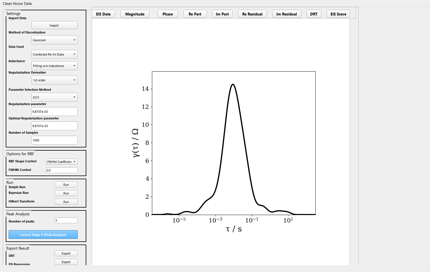
The DRTxECM main window: DRT settings and run buttons on the left, the DRT result gamma(tau) for the ZARC sample data on the right
The actual interface. Running the DRT on the bundled ZARC sample data (81 points, 0.01 Hz to 1 MHz) yields a single relaxation peak in γ(τ), with the regularization parameter selected automatically by GCV. Click the image for full size.

Three-stage workflow

① Import & cleanCSV / TXT, with instrument headers optionally skipped; click on the Nyquist plot to remove noise points; PCHIP interpolation onto a uniform logarithmic frequency grid
→
② DRT → R//CPEMulti-Gaussian peak fitting of the DRT γ(τ), converted automatically into R, C and fc for each peak, and sent to Stage 3 in one click
→
③ ECM fittingZView-style parameter table; LR0 + Σ(Ri//CPEi) circuit; L-BFGS-B bounded optimization; live Nyquist and Bode previews
StageModuleWhat it does
1. Import & clean DataImportPreprocessor
DataCleaningWindow
Flexible CSV / TXT import (rows can be skipped); interactive click-to-remove of noise on the Nyquist plot; PCHIP interpolation onto a uniform logarithmic frequency grid.
2. DRT → R//CPE Gaussian peak decomposition
Stage2Window
Multi-Gaussian fitting of the DRT γ(τ); automatic conversion into RC initial parameters (R, C and fc for each peak); one-click export to Stage 3, starting from R//CPE (initial α = 1.0).
3. ECM fitting CNLS optimization
Stage3Window
ZView-style parameter table; LR0 + Σ(Ri//CPEi) circuit model; L-BFGS-B bounded optimization; live Nyquist and Bode previews; branch-resolved visualization.
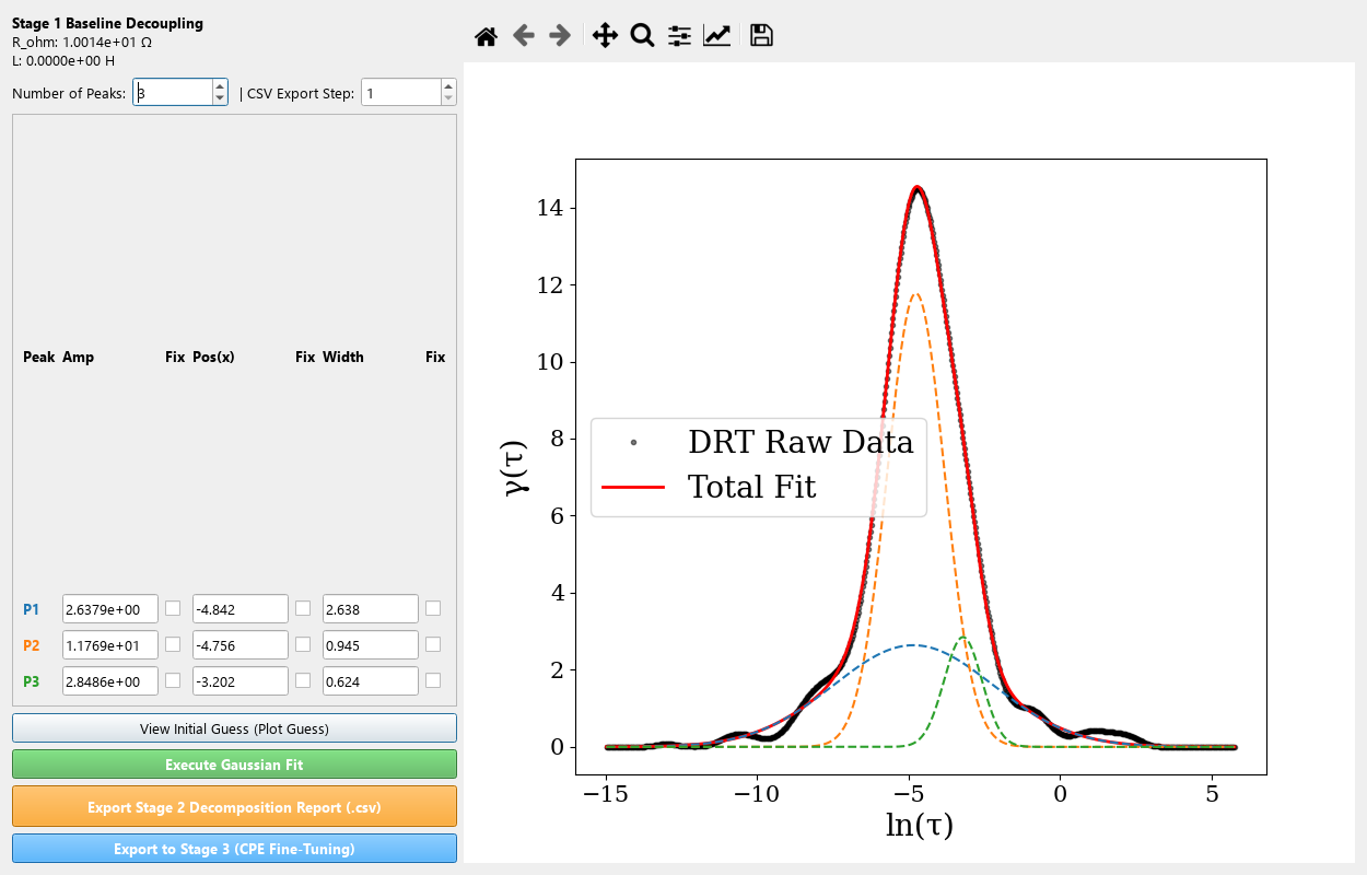
Stage 2: decomposing the DRT gamma(tau) into three Gaussian peaks
Stage 2: decomposing γ(τ) into three Gaussian peaks. The black dots are the raw DRT data, the red line is the sum of the three peaks, and the blue / orange / green dashed curves are the individual peak contributions. Each peak's amplitude, position and width can be locked or released independently.
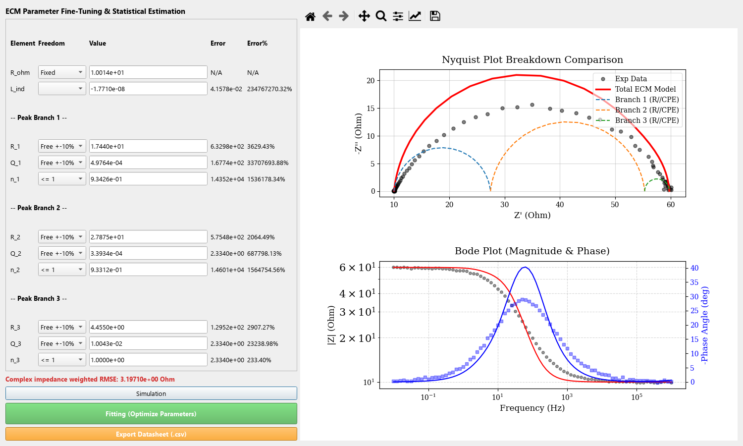
Stage 3: equivalent circuit parameter table, plus branch-resolved Nyquist and Bode plots
Stage 3: R, Q and α for every branch together with the estimated standard errors (Error / Error%), while the Nyquist plot draws each R//CPE branch contribution in a distinct colour. This example deliberately fits a single ZARC semicircle with three branches (over-parameterization), so the standard errors are large — which is exactly what the Error% column is for: telling you whether a parameter is actually constrained by the data.

Key features

CPE phase angle α freely fittedCommercial tools often fix α or restrict it to particular values; DRTxECM optimizes α together with R and Q, bounded by 0.2 ≤ α ≤ 1.05
DRT-informed initial guessThe Gaussian peak parameters are converted directly into physically meaningful starting values, avoiding the convergence problems of random initialization
Branch-resolved visualizationEach R//CPE branch is drawn in a different colour on the Nyquist plot, so their individual semicircle contributions are visible
Interactive data cleaningClick noise points away directly on the plot — no need to go back and edit the raw file
Four DRT algorithmsTikhonov (ridge regression), Bayesian, BHT and GP-DRT, all retained from pyDRTtools
Eight discretization basesGaussian, C2/C4/C6 Matern, Inverse Quadratic, Inverse Quadric, Cauchy, PWL
Seven regularization selection methodscustom, GCV, mGCV, rGCV, LC, kf, re-im
Parameter uncertaintyCovariance estimated from the inverse Hessian matrix, reporting the standard error of every fitted parameter
100% backward compatibleThe original pyDRTtools DRT computation is completely unmodified
Fully offlineAll computation runs on your own computer; data is never uploaded anywhere
Lockable parameter modesEvery R, Q and α can be set to fixed, ±5%, ±10% or free, to simulate the tolerances of real measurements
MIT open sourceAudit it, modify it and build it yourself, commercial use included

Quick start

  1. Download and unzip DRTxECM-win64.zip
  2. Run DRTxECM.exe
  3. Import EIS data (CSV or TXT; instrument headers can be skipped)
  4. Run the DRT (Tikhonov / Bayesian / BHT, whichever you prefer) to obtain γ(τ)
  5. Click Launch Stage 2 to perform Gaussian peak decomposition on γ(τ)
  6. Click Export to Stage 3, adjust R, Q and α, then run the CNLS fit
  7. Export the fitted parameters, the Nyquist and Bode plots, and the contribution of each branch

For fuller operating and interface instructions, see the Guide.

Relationship to pyDRTtools

DRTxECM is not a separate tool rewritten from scratch; it is an extension built on top of pyDRTtools (Ciucci Lab). In the source code, the DRT computations in pyDRTtools/ (Tikhonov regularization, Bayesian, BHT, GP-DRT) are fully retained and unmodified; the additions live in extensions.py and in the Stage 2 and Stage 3 interfaces. This means that the results you obtain at the DRT stage are consistent with using pyDRTtools directly.

If you use DRT computation results in a paper, you must cite the original pyDRTtools publications. The list is compiled under Citation & Credits.

License & source